Analytical Methods

This page provides a summary of the process used to create the models underlying the distribution and abundance maps in the individual Species Accounts. It also gives an overview of the methods that were used to identify the large-scale changes in distribution of the species reported in the Results.

This summary is intended for a general audience; a version with more technical details about the models can be found here.

Purpose of the Models

The Atlas generated two very large avian data sets: one collected by Atlas volunteers and one by field technicians conducting point counts. These data sets were used to create models (mathematical representations/computer simulations) for individual breeding bird species. The models predict species distributions (where they are found on the landscape; using volunteer-collected data) and abundance (in what numbers they are found on the landscape; using point count data) based on underlying environmental characteristics.

The use of models allowed predictions to be made for areas of the state that were not surveyed, painting a more complete picture of distribution and abundance over simply reporting where the species was detected. In addition, we modeled species distributions during the First Atlas and compared them to their distributions during the Second Atlas to assess how they have changed over the 30-year period between Atlases.

Environmental Variables

All models were built in part by using a common set of environmental variables (factors) that represented the topographic, land cover, and climatic variation within the state (Table 1).

Table 1. Environmental variables used in the models and the datasets from which they were derived. The variables were created for all three physiographic regions (Coastal Plain, Piedmont, and Mountains and Valleys), except for Percent Marsh Cover (Coastal Plain only) and Relative Cover of Evergreen Shrubs (Mountains and Valleys only).

Category	Environmental Variable	Source Data Set	Physiographic Region
Topography	Elevation and Latitude Index	National Elevation Dataset	all
Land Cover	Percent Shrubland/Grassland Cover	National Land Cover Database	all
Land Cover	Percent Forest Cover	National Land Cover Database	all
Land Cover	Percent Agricultural Cover	National Land Cover Database	all
Land Cover	Percent Development	National Land Cover Database	all
Land Cover	Percent Marsh Cover	National Wetland Inventory	Coastal Plain
Land Cover	Percent Barren Land	National Land Cover Database	all
Land Cover	Number of Forest Patches	National Land Cover Database	all
Land Cover	Diversity of Habitat Types	National Land Cover Database	all
Land Cover	Size of Largest Forest Patch	National Land Cover Database	all
Land Cover	Relative Cover of Evergreen Shrubs	Sentinel-2 satellite imagery	Mountains and Valleys
Climate	Number of Freezing Days in a Year	Daymet climate datasets	all
Climate	Variation in Annual Rainfall	Daymet climate datasets	all
Climate	Mean Annual Rainfall	Daymet climate datasets	all

Individual land use categories in the National Land Cover Database (NLCD) were combined to create the land cover variables in Table 1. Percent Agricultural Cover includes pasture, hayfields, and cultivated crops. Percent Barren Land typically represents beaches in Virginia. Environmental variables were calculated separately for the First and Second Atlases.

Modeling Breeding Distribution for the Second Atlas

We used occupancy models to predict species distribution for the Second Atlas. The models report the likelihood that a species occurs within, or occupies, each Atlas block (we use the terms ‘occupancy’ and ‘occurrence’ interchangeably). Atlas blocks were the individual units within which bird surveys took place, and each covered approximately 10 mi² (26 km²).

The models used bird data collected by Atlas volunteers at the block level and included all data with at least a “possible” breeding category (see Atlas Methods). We created models for species with sufficient data (more than 50 detections in 20 or more blocks). 

To improve the reliability and accuracy of our predicted distributions, it was important to include in the models the probability (likelihood) of detecting a species. We calculated the probability of detection for each block, incorporating the corresponding number of volunteer hours spent within that block for each year during that species’ breeding season. Survey effort was included because it varied among blocks and, up to a point, greater effort increases the probability of detecting a species if it is present.

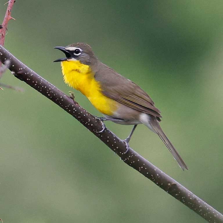
The models identified the important environmental variables within the blocks where a species was detected. For example, the model calculated that Yellow-breasted Chat, a species of open, shrubby habitats, was more likely to be found in blocks with greater shrubland and grassland cover, and blocks with a greater diversity of habitat types, and less likely to be found in blocks with greater forest cover and with larger forest patches. We present the relationships between these variables and occurrence of a species as associationgraphs in the Breeding Distribution section of individual Species Accounts.

The models used these relationships to make predictions about how likely a species is to occur within each block across its core breeding range, whether that be the entire state or one or more physiographic regions (Coastal Plain, Piedmont, Mountains and Valleys; see Virginia Geography and Climate). These predictions were used to create maps representing the species’ distribution (Figure 1). They are found in the Breeding Distribution section of individual Species Accounts.

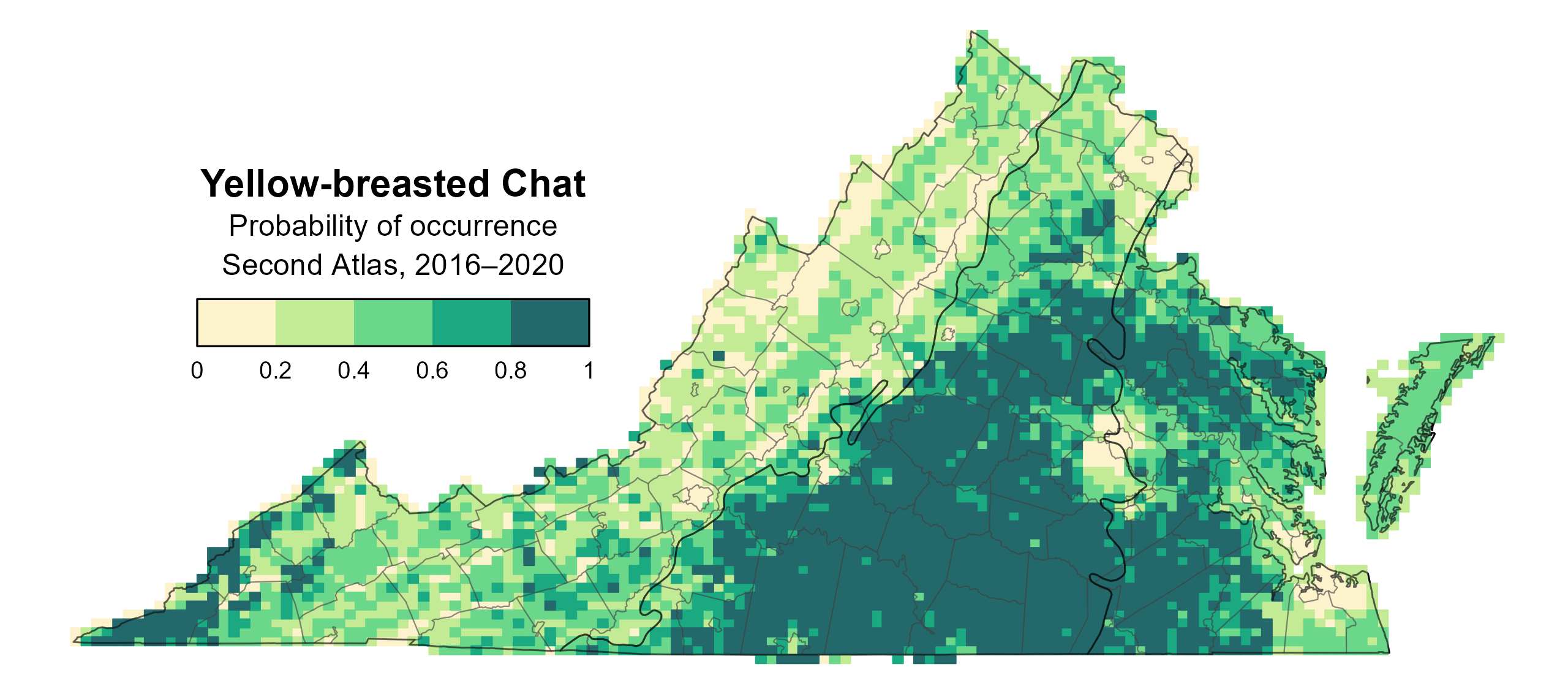
Figure 1. Yellow-breasted Chat breeding distribution based on probability of occurrence (Second Atlas, 2016–2020). This map indicates the probability that this species will occur in an Atlas block based on environmental variables and after adjusting for probability of detection.

Predicted occurrence can range between 0 and 1, which can be interpreted as a 0-100% chance of a species occurring within a block. In Figure 1, the darker green blocks are those with an 80-100% chance of Yellow-breasted Chat occurring within the block. Though the chat has a statewide distribution, the map indicates that it is most likely to be found in areas of the southern Piedmont, inner Coastal Plain and Cumberland Mountains. Species with models with weak relationships between occurrence and the environmental variables may not have many blocks with a high likelihood of occurrence.

Evaluating Change in Distribution Between Atlases

We estimated changes in species distribution between Atlases by comparing distribution maps based on occupancy models for the Second Atlas to those for the First Atlas. Because we had less data for the First Atlas and were unable to factor in volunteer survey hours (due to inconsistent reporting), we adopted a coarser modeling approach to estimate probability of detection.

Detection probability, along with bird data and the environmental variables were used to create models that assigned a probability of occurrence to each block that was surveyed. We repeated this modeling process using Second Atlas data so that model outputs would be comparable between Atlases.

Using the models, we subtracted the probability of occurrence for the First Atlas from that for the Second Atlas on a block-by-block basis to estimate change in species distribution between Atlases. This was done only for those blocks that were surveyed in both Atlas periods. Maps of change in distribution are presented in the Breeding Distribution section of the Species Accounts.

On the maps, the change in the likelihood of a species occurring in a block is considered constant when the predicted change is between -0.3 and 0.3, moderate when it is between -0.5 and -0.3 or 0.3 and 0.5, and substantial when it is between -1.0 and -0.5 or between 0.5 and 1.0.

We visually evaluated the maps of change in distribution to assess whether distributions had changed at the scale of the three physiographic regions (see Results). We looked for strong signals of change in the form of extensive, clumped distributions of blocks with moderate or substantial change throughout one or more regions. The map for Yellow-breasted Chat shows a striking decline in the probability of the species occurring across the entire Mountains and Valleys region. This indicates that its distribution west of the Blue Ridge has contracted since the First Atlas (Figure 2).

Figure 2. Yellow-breasted Chat change in breeding distribution between Atlases based on probability of occurrence. Blocks with no change (tan) may have constant presence or constant absence.

For species with less obvious patterns, we compared the proportion of blocks with change relative to those with constant occupancy after removing blocks with a low probability of occurrence (i.e. less than 0.3) in both Atlases. We considered there to be regional level change when 60% or more of blocks showed change between Atlases.

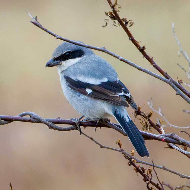
For species without maps of change in distribution, we turned instead to their breeding evidence maps. We considered significant contractions in distribution to have occurred when species were reported in a minimum of 50 fewer blocks during the Second Atlas and when that translated to a greater than 50% decline in the number blocks from the First Atlas. For example, Loggerhead Shrike (Lanius ludovicianus) was reported from 94 fewer blocks during the Second Atlas (Figure 3), which represented a 67% decline in the number of blocks from the First Atlas. Survey effort during the Second Atlas was two to five times greater and more geographically widespread than during the First. Therefore, a compelling case can be made that species detected in significantly fewer blocks during the Second Atlas have indeed seen a negative impact to their breeding distribution.

Figure 3. Loggerhead Shrike breeding observations from the First and Second Atlas. 

Modeling Abundance and Estimating Population Size for the Second Atlas

We used the Atlas point count data set to model abundance (number of individuals) and estimate total population size in the state for species that were detected at 50 or more point count locations. We included only detections within 100 m of the survey points, as many forest species are difficult to detect beyond that distance. We combined the point count bird data with probability of detection and the environmental variables (scaled to 1 km²) into models that produced values of predicted abundance for a species. The maps resulting from these models (Figure 4) are found in the Population Status section of individual Species Accounts.

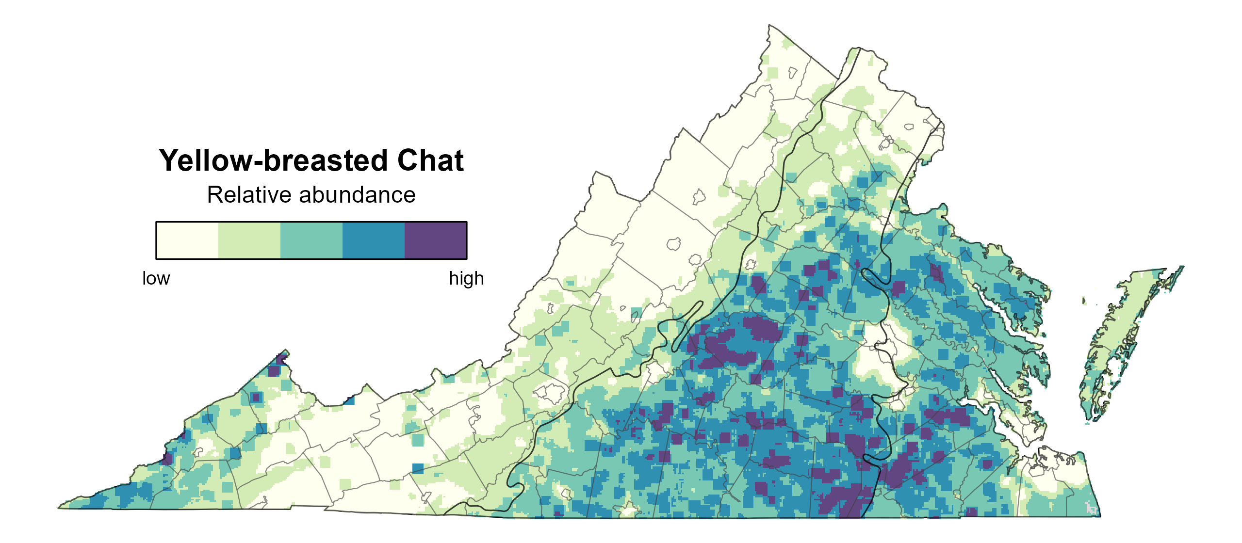
Figure 4. Yellow-breasted Chat relative abundance (Second Atlas, 2016–2020). This map indicates the predicted abundance of this species at a 0.4 mi² (1 km²) scale based on environmental variables and after adjusting for probability of detection.

To estimate total breeding population size for a species, we averaged predicted abundance values at the 1 km² scale to get a single value (plus confidence interval). We then multiplied that value by the total area in the relevant physiographic region. Population estimates should be interpreted as the predicted number of detectable individuals.  Population estimates are rounded to the nearest thousand and represent the predicted number of detectable individuals*, rather than the total number of individuals. We also provide the upper and lower range within which there is 95% confidence that the true population size falls.

*Detectable individuals are the number of individuals expected to be detectable during surveys, rather than the true total number of individuals present. This is because there may be sex biases in singing/calling rates for many species (mostly songbirds) that were detected only via their vocalizations during the surveys. There is a growing body of evidence that females sing more than previously thought (Odom et al. 2014). We did not correct for those biases because we do not have good estimates for what those are. 

---

Literature Cited

Odom, K. J., M. L. Hall, K. Riebel, K. E. Omland, and N. E. Langmore (2014). Female song is widespread and ancestral in songbirds. Nature communications 5:3379.