Models

This page provides a summary of the process used to create the models underlying the distribution and abundance maps in the individual Species Accounts. It also gives an overview of the methods for identifying the large-scale changes in distribution of the species reported in the Results page.

Covariates

To create distribution (occupancy) and abundance models for species with sufficient data, we used environmental covariates that represented the topographic, land cover, and climate variation within the state.

For land cover data, we used the 2016 30m National Land Cover Dataset (NLCD) (Dewitz 2019) to create percent cover variables for agriculture (pasture/hay and cultivated crops), barren (typically, beaches), developed, early successional (shrub/scrub and grassland/herbaceous), forest, water, and wetland cover types. We calculated the diversity of land cover types within a block (approximately 26 km² [10 mi²]; for distribution models) or 1 km² cell (0.39 mi²; for abundance models) using the Modified Simpson’s Diversity Index (MSIDI) (Simpson 1949; McGarigal et al. 2023).

To examine forest configuration variables, we calculated the number of NLCD forest patches and the largest patch index (LPI) using the “queen’s case” of all 8 neighboring cells to define patches (McGarigal et al. 2023). For the mountain physiographic regions (Blue Ridge Mountains, Northern Ridge and Valley, Northern Cumberland Mountains, Southern Cumberland Mountains), we also created a variable to represent the percent cover of evergreen shrubs. We calculated this Enhanced Vegetation Index (EVI) for the period of leaf-off (mid-November to mid-March) using Sentinel-2 10m (32.8 ft) satellite imagery for the years 2018–2020 (2018 is the first year Sentinel-2 imagery is available), and then averaging those values across years.

For the Coastal Plain physiographic region, we also created a “marsh” covariate that better represented salt and brackish marshes than the NLCD dataset. We used the National Wetland Inventory data (downloaded in fall 2023) on estuarine, intertidal, emergent wetlands (code E2EM) to calculate the percent combined cover of salt and brackish marshes.

For topographic information, we used the National Elevation Dataset to generate a Relative Phenology Index (RPI) that represented both elevation and latitude and longitude (Hopkins 1920). For climate data, we used the Daymet 1km (0.62 mi) daily gridded climate datasets from 2016–2021 (Thornton et al. 2022) to calculate several climatic variables at a yearly scale and then averaged them across the 5-year time span of the Second Atlas (2016–2020). The climatic variables included:

• Mean annual precipitation,
• Variation of annual precipitation (standard deviation),
• Total summer (May–July) precipitation,
• Number of freezing days in a year,
• Number of days with temperatures above 25º C (77 º F) in a year,
• Number of days with temperatures above 30º C (86 º F) in a year, and
• Growing degree days (GDD; mean temperature is >0º C (32º F).

The volunteer-collected Atlas data and the Atlas point count data (see Atlas Methods) were collected at different geographic scales, so we aggregated covariate information to best match those scales. For occupancy analyses that used the volunteer dataset, which was collected at the block level, we aggregated covariates by summing (landcover variables), averaging (climate variables, EVI and RPI) or directly recalculating them (MSIDI and LPI) at the block level.

For point count datasets that were collected at a much finer scale (100m [328 ft] radius counts), we wanted to match the scale of covariate information as best as possible to be able to make the most accurate predictions of total abundance. However, the minimum resolution of our covariate dataset was 1 km² (for the Daymet dataset), so we aggregated to 1 km² grid cells for abundance analyses.

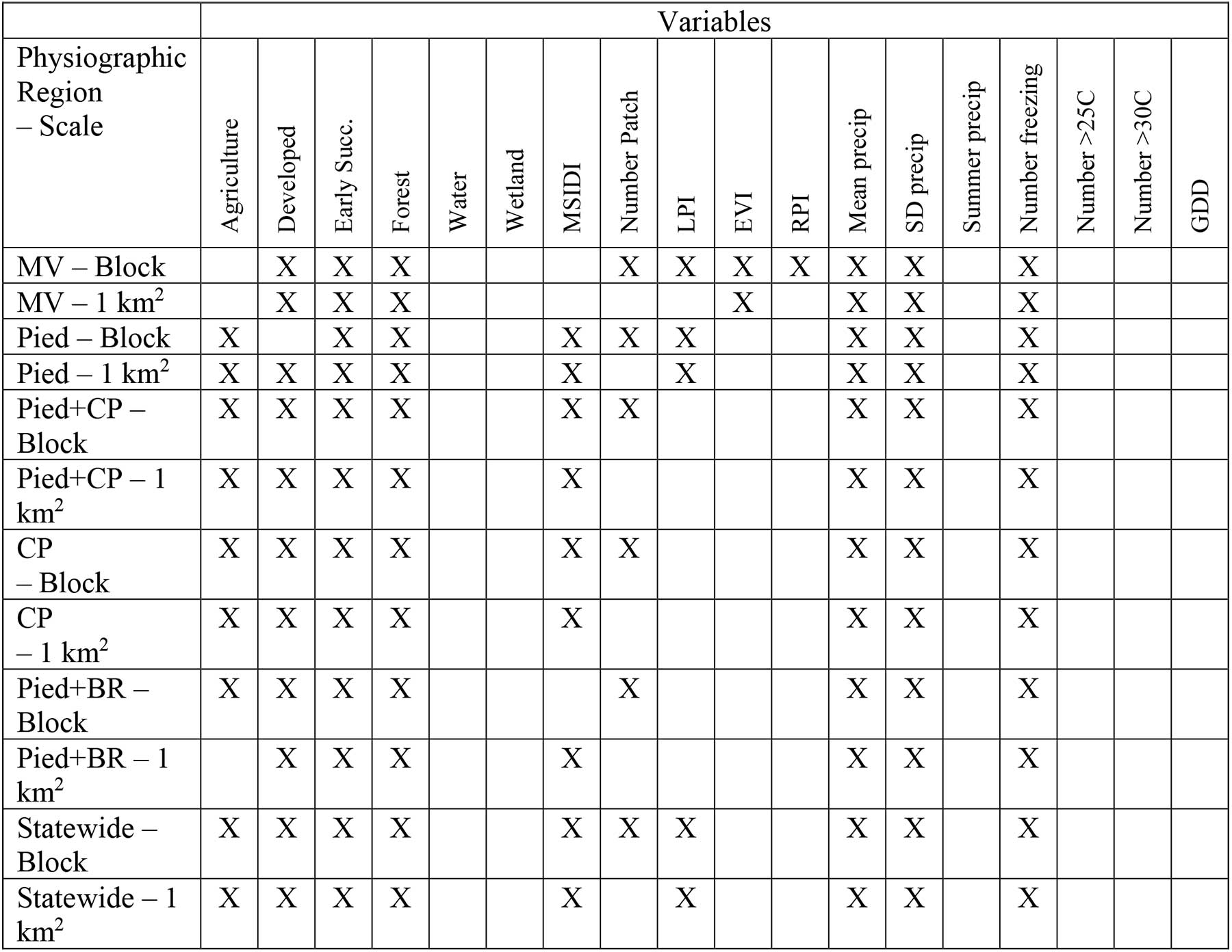
The set of covariates included many that were highly correlated with each other, and correlated variables cannot be included in the same model together. For each physiographic region group, we examined the correlations and removed variables to create a set of uncorrelated variables (using a |r|<0.6 correlation threshold) for each physiographic region and each scale (block scale, and 1 km² scale).

Physiographic regions were those delineated by the Virginia Department of Wildlife Resources (VDGIF 2005), and for analysis, we grouped these into six physiographic region groups:

• Mountains and Valleys (Blue Ridge Mountains, Northern Ridge and Valley, Northern Cumberland
• Mountains, and Southern Cumberland Mountains),
• Piedmont (Southern Appalachian Piedmont),
• Piedmont plus Coastal Plain (Southern Appalachian Piedmont, Middle Atlantic Coastal Plain),
• Coastal Plain (Middle Atlantic Coastal Plain),
• Piedmont plus Blue Ridge (Southern Appalachian Piedmont, Blue Ridge Mountains), and
• Statewide species (all physiographic regions).

Table 1. List of uncorrelated variables (marked with X) used in occupancy (“Block” scale) and abundance (1 km2 scale) models. Each row indicates the physiographic region (MV=Mountains and Valleys), Pied=Piedmont, BR=Blue Ridge, CP=Coastal Plain, Statewide) and scale. Additional covariates were used for some CP species that rely heavily on marshes and beaches (see main text). 

To improve model estimation efficiency, we scaled covariate values to be approximately between 0 and 1 and back transformed to the original value scale for environmental associations figures showing covariate effects (see individual Species Accounts). We did not standardize covariates, which would have allowed direct comparison of effect sizes among covariates, because we needed to be able to apply estimated relationships between environmental covariates and either occupancy or abundance to unsampled blocks to create full physiographic region maps of predicted occupancy and abundance.

The above methods for developing covariates were repeated for the First Atlas (1984–1989; note that the First Atlas officially took place 1985–1989, but a pilot year in 1984 generated 10% of the bird data used in the models). The NLCD dataset used was from 2001 (the earliest available landcover dataset that was comparable to the 2016 NLCD dataset at the time of download), and NLCD forest data were used to calculate number of forest patches and LPI. The EVI variable could not be calculated for this time period as full coverage satellite imagery was not available. The Daymet climate dataset was available and used for the First Atlas time period.

Occupancy Models

To model species distribution (occupancy) for the Second Atlas, we used the volunteer dataset collected at the block level, using all data with at least a “possible” breeding category. We created models for species with sufficient data (>50 detections in 20+ blocks). We assumed that occupancy is fixed over the 5-year period of the Atlas and that every year that a block was visited is an independent test of whether the species could be detected. In that way, we were able to account for imperfect detection and improve the reliability and accuracy of occupancy maps over simply reporting the blocks in which a species was detected.

We modeled the probability of detecting a species as a function of the number of volunteer hours spent within a block, during the period corresponding to that species’ breeding season, in each year. We only modeled species within the three major physiographic regions (Coastal Plain, Piedmont, and Mountains and Valleys) that represent the known core of their breeding range.

We estimated the probability of occupancy using the unmarked package (Fiske 2011) in program R v. 4.2.1 (R Core Team 2021) using the occu function. We created all possible linear models of the covariates (excluding interactions), as well as a null model (intercept only). We compared models using Akaike’s Information Criterion corrected for small sample sizes (AICc). To account for model uncertainty, we averaged all models that contributed to 95% of the total model weight and kept variables with a model-averaged 95% confidence interval that did not overlap zero.

We then created a “top” model using those covariates and used that top model to predict occupancy probability for all blocks within the physiographic region. We assessed model fit using the Area Under the Receiver Operating Characteristic Curve (AUC) scores. However, as traditional methods of calculating AUC do not account for imperfect detection (Zipkin et al. 2012), we used a modified approach of calculating AUC following the methods of Ceradini et al. (2021). We only interpreted models that had an AUC ≥ 0.7, which is considered a model with acceptable abilities to discriminate between an occupied and unoccupied block.

We created maps of predicted occupancy by applying the estimated relationships between occupancy and covariates back to maps of the covariates (landcover, climate, etc.), only for the relevant physiographic regions for a species. The predicted probability of occupancy can range between 0 and 1, which can be interpreted as a 0 or 100% chance of a block being occupied. Species with models with poorer predictive capabilities may not have many blocks with high predicted occupancy probabilities, which simply means that the relationships with covariates were weak.

Change in Distribution (Occupancy) Between Atlases 

The data reporting process for the First Atlas was substantially different from the Second Atlas. In order to assess change in occupancy status, we needed to put the datasets on the same footing and analyze them the same way. Data for the First Atlas included only the year in which the species was first recorded for each block, but not whether it was detected in later years. Thus, we could not use the “years as visits” model that we used above. By including records with ‘observed’ and ‘flyover’ breeding codes to boost sample size, we were able to use a “time-to-detection” (TTD) model because approximately one-third of the blocks were visited in more than one year. We therefore could estimate the probability of detection by estimating the time to first detection (Kery and Royle 2016).

We did not include any detection covariates as number of survey hours was not systematically reported in the First Atlas. We used the unmarked function occuTTD to create the models and used the same process as above to choose top models. We also conducted this process using Second Atlas data to be able to compare outputs that were both derived from TTD models; we did not include records with ‘observed’ or ‘flyover’ breeding codes, as sample sizes were already sufficient.

We again used AUC to evaluate model predictive power, but due to data limitations, we reduced the threshold cut-off for interpretation to AUC ≥ 0.6. We calculated the change in occupancy as the difference in predicted probability of occupancy between Atlases, only for those blocks that were surveyed in both Atlas periods. In maps of this occupancy change, “constant” is when the predicted change is <0.3, a moderate amount of change is between 0.3–0.5, and a substantial amount of change is for values >0.5.

We conducted a visual evaluation of occupancy change maps to assess whether distributions had changed at the scale of the three main physiographic regions. We first looked for strong signals of change in the form of extensive, clumped distributions of blocks with change >0.3 throughout one or more regions. For species with less obvious patterns, we quantified the proportion of blocks with change relative to those with constant occupancy after removing blocks that were unoccupied (occupancy probability <0.3) in both Atlases. We set a threshold of 60% of blocks with change as representative of change at the regional level. We did not consider model AUC scores.

For species without occupancy change maps, we quantified the difference in blocks with breeding evidence between Atlases. We considered significant contractions in distribution to have occurred when species were reported in 50+ fewer blocks during the Second Atlas, and when that translated to a decline of >50% in the number blocks from the First Atlas. For example, Loggerhead Shrike (Lanius ludovicianus) was reported from 94 fewer blocks during the Second Atlas, which represented a 67% decline in the number of blocks from the First Atlas.

For these species we also visually evaluated the distribution of the change to assess whether it was occurring at the regional level, as we had done for species with occupancy change maps. Interpretation of these raw, unmodeled data is less reliable than interpretation of the occupancy change maps because survey effort is uneven among individual blocks and between Atlases; this can affect whether a species that is present in a block is detected.

=Survey effort during the Second Atlas was two to five times greater than during the First; this also translated to superior geographic coverage, especially in the Mountains and Valleys region and in the southern Piedmont. Therefore, a compelling case can be made that species detected in significantly fewer blocks during the Second Atlas have indeed seen a negative impact to their breeding distribution.

Abundance Models

We used the Atlas point count dataset to model abundance and estimate total population size in the state for species that were detected at 50+ point count locations. We thresholded detections to only those within 100 m of the survey points, as for many forest species, detection is very limited beyond that distance. To account for imperfect detection, we again used a TTD model (package unmarked nmixTTD function) with the time of first detection being the minute the species was detected in the five minutes of the point count (see point count protocol for more details). For detection covariates, we used noise level (which was correlated with wind) and an observer experience score (1–3, with 3 being most experienced). 

We used the same process of creating models and selecting the top model as described above, but at a scale of 1 km2. However, our process for evaluating model fit and validity varied slightly, given that the AUC methods used for occupancy models are not appropriate for abundance model evaluation. Instead, we used the following criteria to evaluate abundance models: (a) congruity in predictions between occupancy and abundance models and (b) a minimum of one significant (p <0.01) predictor of abundance (otherwise a prediction is not driven by any relationships). 

To predict total breeding population size for the species in the modeled physiographic regions, we calculated the predicted abundance for each point count location using the top model (doing this accounted for imperfect detection). We then multiplied the predicted abundance for each point count location (mean and 95% confidence interval) by a correction factor of 31.847 (to convert expected counts in a 100m radius circle to a 1 km2 square cell). We averaged the resulting values to get a single value (plus confidence interval) which we then multiplied by the total area in the relevant physiographic region (e.g., 110,785 km2 [42,774 mi2] for statewide species). 

Total abundances should be interpreted as the predicted number of detectable individuals. We did not correct for sex or age ratios, as we did not have sufficient data to do so, and existing correction factors are likely biased given the growing body of evidence that females sing more than previously thought (Odom et al. 2014). 

---

Literature Cited

Ceradini, J., D. Keinath, I. Abernethy, M. Andersen, and Z. Wallace (2021). Crossing boundaries in conservation: Land ownership and habitat influence the occupancy of an at‐risk small mammal. Ecosphere 12:e03324. https://doi.org/10.1002/ecs2.3324
Dewitz, J. (2019). National land cover database (NLCD) 2016 products (ver. 3.0, November 2023): U.S. Geological Survey data release. https://doi.org/10.5066/P96HHBIE.
Fiske I., and R. Chandler (2011). Unmarked: an R package for fitting hierarchical models of wildlife occurrence and abundance. Journal of Statistical Software, 43:1–23. https://www.jstatsoft.org/v43/i10/.
Hopkins, A. D. (1920). The bioclimatic law. Journal of the Washington Academy of Sciences 10:34–40.
Kery, M., and J. A. Royle (2016). Applied hierarchical modeling in ecology, volume 1. Academic Press.
McGarigal K., S. A. Cushman, and E. Ene (2023). FRAGSTATS v4: spatial pattern analysis program for categorical maps. https://www.fragstats.org.
Odom, K. J., M. L. Hall, K. Riebel, K. E. Omland, and N. E. Langmore (2014). Female song is widespread and ancestral in songbirds. Nature communications 5:3379.
R Core Team (2021). R: A language and environment for statistical computing. R Foundation for Statistical Computing, Vienna, Austria. https://www.R-project.org/.
Simpson, E. H. (1949). Measurement of diversity. Nature 163:688.
Thornton, M. M., R. Shrestha, Y. Wei, P. E. Thornton, and S. C. Kao (2022). Daymet: daily surface weather data on a 1-km grid for North America, version 4 R1. ORNL DAAC, Oak Ridge, TN, USA. https://doi.org/10.3334/ORNLDAAC/2129.
Virginia Department of Game and Inland Fisheries (VDGIF) (2005). Virginia Wildlife Action Plan. Virginia Department of Wildlife Resources, Henrico, VA, USA.
Zipkin E. F., E. H. Campbell Grant, and W. F. Fagan (2012). Evaluating the predictive abilities of community occupancy models using AUC while accounting for imperfect detection. Ecological Applications, 22:1962–1972.